🚀 Setup & Usage

This section shows you how to run RegionMatch in practice, covering installation, execution via CLI and Python API, parameter configuration, and interpretation of the output.

If you are mainly interested in the conceptual background, see General Overview.

1. Installation and Environment

RegionMatch is available as a Freva plugin and runs within a Freva-enabled environment.

1.1 Load required modules

module load clint regiklim-ces

1.2 Requirements

access to a Freva instance (e.g. RegIKlim)
a valid Freva project and product
no additional local installation required

2. Running RegionMatch

RegionMatch can be executed either via Command Line Interface (CLI) or the Python API. Both produce equivalent results.

2.1 Command Line Interface

module load clint regiklim-ces

freva-plugin regionmatch \
    region="Spree-Neiße" \
    sociodemographic_weight="0.5" \
    climate_weight="0.5" \
    orographic_weight="0.5" \
    landuse_weight="0.5" \
    number_of_similar_regions=10

This configuration:

uses Spree-Neiße as the reference region
assigns equal relevance to all four aspects
returns the 10 most similar districts

2.2 Python API

import freva

plugin_values = {
    region="Spree-Neiße",
    sociodemographic_weight="0.5",
    climate_weight="0.5",
    orographic_weight="0.5",
    landuse_weight="0.5",
    number_of_similar_regions=10
}

freva.run_plugin("regionmatch", **plugin_values)

The Python API prints the paths to the generated output files.

3. Parameters

Required

region : str , default: undefined
The NUTS3 region (district) in Germany to be used as reference. Region names are based on a shapefile from the Bundesamt für Kartographie und Geodäse and listed in assets/district_list.py.

sociodemographic_weight : float, default: undefined
Numeric input that defines the relevance of the sociodemographic aspect in the similarity calculation. Users must provide a value from the set of allowed weights.

Valid values:

0 → No relevance
0.5 → Medium relevance
1 → High relevance

climate_weight : str, default: undefined
Relevance of the climate aspect in the similarity calculation. Same valid values as above.

orographic_weight : str, default: undefined
Relevance of the orographic aspect in the similarity calculation. Same valid values as above.

landuse_weight : str, default: undefined
Relevance of the land use aspect in the similarity calculation. Same valid values as above.

Optional Parameters

number_of_similar_regions : int, default: 10
Number of similar regions (excluding the selected one) to return.

extra_scheduler_options : str, default: none
Additional options for job submission to the workload manager (comma-separated). Only applicable in batch or web mode.

caption : str, default: none
Optional caption to be displayed with the result image.

unique_output_id : bool, default: True
If True, appends the Freva run ID to the output folder name to ensure uniqueness.

4. Output

RegionMatch returns:

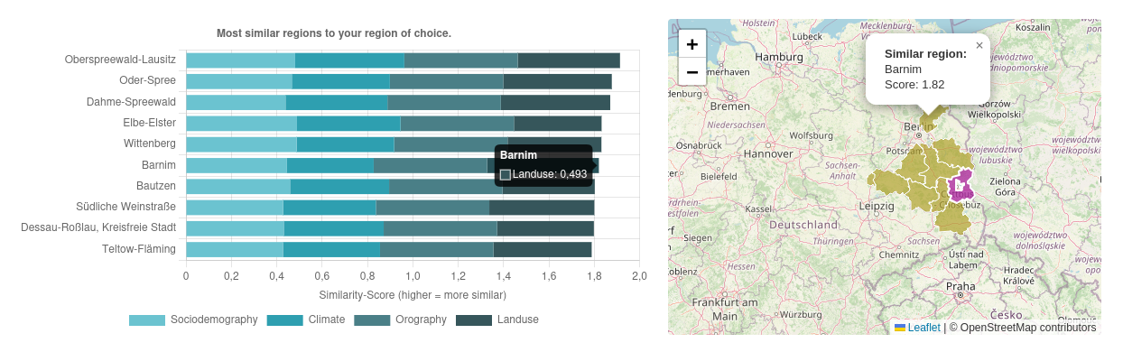
A dynamic dashboard (requires Freva GUI: RegIKlim) combining:
- a boxplot of similarity scores and aspect contributions for the top N similar regions
- a map highlighting the reference region and the top N similar regions
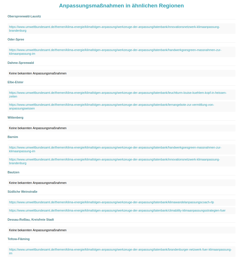
A list with links to already implemented adaptation measures (requires Freva GUI: RegIKlim).
A .zip file containing:
- a static figure regionmatch_results_figure_<NUTS_CODE>_<sociodemography_weight>_<climate_weight>_<orography_weight>_<landuse_weight>.png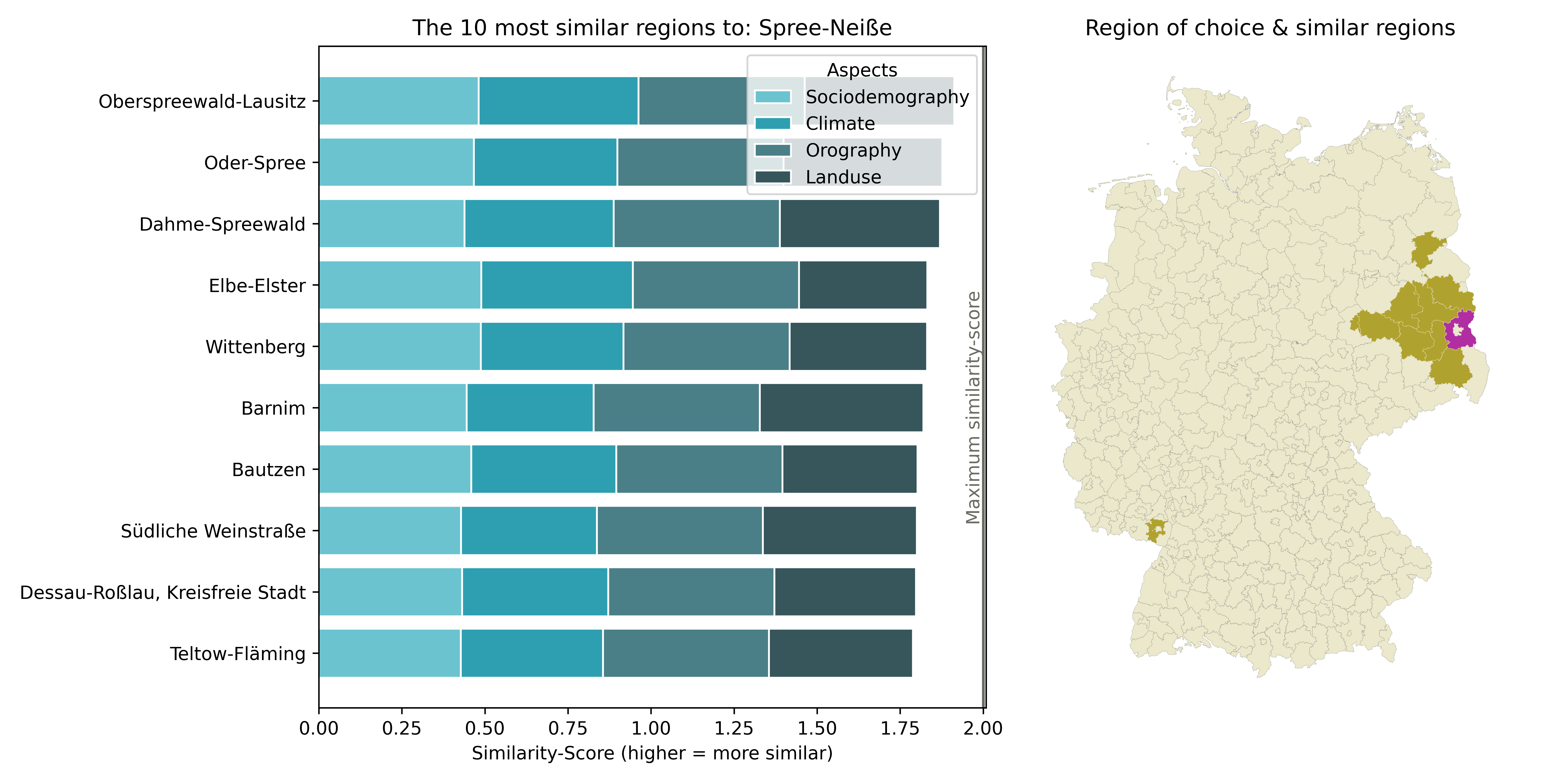
- a data table regionmatch_results_table_<NUTS_CODE>_<sociodemography_weight>_<climate_weight>_<orography_weight>_<landuse_weight>.csv

Example: For Spree-Neiße with all aspects weighted at medium relevance, the table file would be: regionmatch_results_table_DE40G_0.5_0.5_0.5_0.5.csv

4.1 Explanation of the CSV Table

The CSV file contains the raw data for the target region and the top N similar regions

Column name	Description
`NUTS_NAME`	Name of the region
`NUTS_CODE`	ID of the region
`total_size`	Total area in km²
`total_population`	Total population
`population_density`	Population density
`city_and_traffic`	Share of urban and transport areas (%)
`agriculture`	Share of agricultural land (%)
`forest`	Share of forest area (%)
`population_older_65y`	Share of population aged 65 and older (%)
`orography_type`	Orography type
`txge30_historical`	Number of hot days within a year as historical average
`txge30_ssp370-gwl2k`	Change of hot days in a 2 °C warmer world
`txge30_ssp370-gwl3k`	Change of hot days in a 3 °C warmer world
`r30mm_historical`	Number of heavy precipitation days within a year as historical average
`r30mm_ssp370-gwl2k`	Change of heavy precipitation days in a 2 °C warmer world
`r30mm_ssp370-gwl3k`	Change of heavy precipitation days in a 3 °C warmer world
`cdd_historical`	Longest dry spell within a year as historical average
`cdd_ssp370-gwl2k`	Change of longest dry spell length in a 2 °C warmer world
`cdd_ssp370-gwl3k`	Change of longest dry spell length in a 3 °C warmer world
`tr_historical`	Number of tropical nights within a year as historical average
`tr_ssp370-gwl2k`	Change of tropical nights in a 2 °C warmer world
`tr_ssp370-gwl3k`	Change of tropical nights in a 3 °C warmer world
`similarity_score`	Score describing the similarity
`share_sociodemography`	Contribution of the sociodemographic aspect to the similarity score
`share_climate`	Contribution of the climate aspect to the similarity score
`share_orography`	Contribution of the orography aspect to the similarity score
`share_landuse`	Contribution of the land use aspect to the similarity score
`adaptation_measures`	Links to implemented adaptation measures (semicolon separated)

Notes on interpretation

The similarity scores reflect the sum of weighted contributions from the four aspects (climate, sociodemography, orography, land use). Higher scores indicate regions that are more similar to the reference region.
Aspect-specific contributions are relative to the chosen weights, allowing you to see which aspects drive the similarity for each region.
The indicators calculated from regional climate model data are ensemble mean values (average over nine model simulations, see NUKLEUS model data for details).
- historical: 1961–1990
- ssp370-gwl2k: 30-year period in which global warming reached 2 K on average based on the SSP3-7.0 scenario
- ssp370-gwl3k: 30-year period in which global warming reached 3 K on average based on the SSP3-7.0 scenario

Next Steps

Learn about the underlying maths in Background Theory
Revisit the conceptual foundations in General Overview